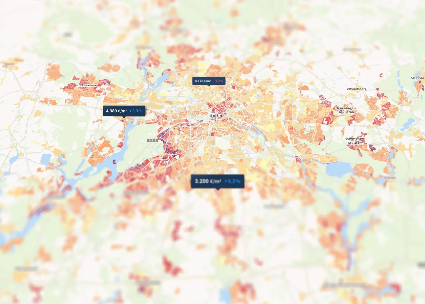
Property price trends
How does the property price explorer work? What is there to consider from a technical perspective?
Introduction
It is of crucial importance to make a precise and an adequate property price estimate. Under- or over-evaluation can lead to wrong business decision, losing money or extraordinary long selling time. On the other hand, having an accurate estimate of a property and knowing trend developments of real estate prices, helps sellers or investors in maximizing their profits. In this article we would like to address how we, at Homeday, solved the technical sides of the following three problems:
Automatic property evaluation; automatic valuation method (AVM)
Monthly property price trend generation for a city, district or zip code
Monthly estimation of a price trend on a building block level
For automatic property evaluation we use state-of-the-art algorithms from Machine Learning field. To the best of our knowledge, we are the first to deploy such sophisticated methodologies in real estate German market.
Problems and solutions
Automatic property evaluation
Affordability of apartments or houses serves as a proxy of a macro-economic activity. For this reason, monitoring real estate property price developments, i.e. price trends, is very important for various groups of stakeholders within the real estate industry. Serving also as an indication of financial stability, it plays a pivotal role in a citizens’ decision whether to buy or sell a property. Usually, development of the price of an “average” property is used as an approximation for the price trend.
Nevertheless, trends can serve only as an approximation, guidance for estimating the exact price of a property. The exact price will largely depend on the exact location, neighborhood characteristics (e.g., proximity to public transport, restaurants, parks), property specific attributes (e.g., construction year, number of rooms, living space area, interior condition), macro- and microeconomic factors, pollution, etc.
Needless to say, property appraisal is a challenging problem and doing it automatically is particularly challenging. Firstly, it is a non trivial task to gather enough relevant transactional data that spans a substantial period and has rich data variability. Secondly, the method should cope with missing data (e.g., some properties might have a missing construction year etc.). Third, it should be scalable. Fourth, it should be easy to interpret results, so it will be easier to adjust price afterwards, if needed. Finally, it should be as precise as possible, ideally with very small error rates for a large group of properties.
Solution
We developed an automatic valuation method for apartments and houses that spans all of Germany, including rural regions with as few as 30 properties. It allows us to estimate the price (aka, HOMEDAY-PREIS) of any property in Germany within the last 5 years. The idea behind it is to simulate hundreds of thousands of human professional appraisers estimating prices for all properties in the dataset and then averaging their estimations, $$$ x_\text{estimate} = \frac{1}{N} \sum_{i=1}^{N} Appraiser_i (\mathbf{b}_{property}) %0 $$$
Equation 1: Exemplary derivation of an automatic appraisal.
Eq. 1 illustrates a summary of the automatic appraisal method, where vector $$ \mathbf{b}_{property}%0 $$ denotes the vector of attributes of a property, $$ Appraiser_i %0 $$ stands for $$ i%0 $$-th simulated professional appraiser, and scalar $$ x_\text{estimate} %0 $$ denotes the final appraisal result. We need to note, that the result will be the logarithm of the price, i.e. $$ \exp (x_{estimate})%0 $$ will be the actual estimate. Applying $$ \log%0§ $$ function on prices when processing them fixes positive-skewness of price distribution (see Figure 1 for an example). The detailed analysis of all the preprocessing and cleaning steps would go beyond the scope of this article.
The current accuracy table for biggest cities can be found in our Preisatlas information; it is regularly updated with the improvement of the algorithm.
Monthly trend generation
Tracking price changes of an “average” property on a monthly basis is an approximation for the property price trend. The trend can be approximated by taking the mean price of all properties sold within a given period of interest.
However, since the price distribution of properties is positively skewed (see Fig. 1) and to reduce the influence of luxury properties, the median and not the mean of the sold properties is considered as the price trend.
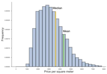
Figure 1: Example of a positively skewed distribution square meter prices of apartments sold in Berlin (2016).
Unfortunately, this approach has several major drawbacks and technical challenges which need to be addressed. Firstly, it provides a noisy estimate, since properties that actually were traded in different periods are usually not representative (a small fraction of all properties was actually traded) and are different. The approach is also prone to bias, i.e. a systematic error, either because the quality of all properties is changed or if some type of properties are sold more frequently.
Additionally, if the considered period is long enough and the resolution is a country or a big residential area, a median estimate is usually a reliable estimation. Moreover, commonly used property price indexes produce similar results (see [5] for details and thorough overview of different property price index derivations). However, when we increase frequency, i.e. monthly, and increase resolution, e.g., to zip code, district, or, even, a building block, the task of determining the price trend becomes extremely challenging (see Fig. 2: note in one month the median is 10.000€/sqm, whereas in another 4.000€/sqm). This is due to fact that there is almost no transaction data, i.e. no properties were sold, great differences in quality of sold properties. Finally, it is a challenging task to gather data on such a low resolution level.
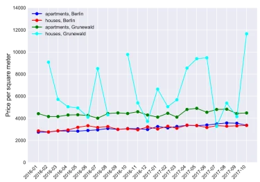
Figure 2: Median prices of sold properties in all of Berlin and its district Grunewald, calculated monthly. Note that due to the low number or the absence of sold properties, the estimation is unreliable or can not be calculated.
Solution
To overcome the previously mentioned challenges related to frequency sampling, we proposed the HOMEDAY-TREND, a novel method to estimate real estate price trends on the German real estate market. We use hedonic imputation with quality-change adjustments to estimate the price trends similar to the model used by Zillow, the number one real estate service company from the US.
The HOMEDAY-TREND algorithm was used for calculating the price trends for all zip codes on our Homeday Preisatlas. Note, its power comes especially to prominence for rural areas, since with even little transactional data for each particular period (e.g., price trend in Huy city), we were still able to produce reasonable estimates. Moreover, we can estimate trends on a monthly basis and not quarterly basis, as displayed on the HOMEDAY-PREISATLAS. Our calculated trends are:
bias free,
applicable to any resolution level (country, city, district, zip code),
applicable to any frequency (monthly, quarterly, annually, etc.),
and seasonally adjusted.
The restricting factor is that there has to be a minimal number of properties (e.g., 30), present in the resolution level, to be considered.
Questions related to price trend time series smoothing, seasonality effects adjustments and others, though addressed in our approach for derivation of all trends, are beyond the scope of this article (see [7] for an introductory discussion of the mentioned problems).
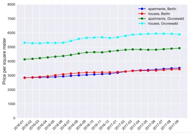
Figure 3: Trends generated for apartments and houses in Berlin and district Grunewald. Compare to Figure 2, the original cleaned raw data.
Estimation of a price trend on a building block level
Given monthly price trends on district or zip code levels, how can we estimate trends on a building block level? This is a not trivial problem and it cannot be solved exactly due to the lack of sufficient transactional data. One should resort to an approximate estimation by considering the quality of each building block (socio-demographic data), geographical data (proximity to parks etc.) and other related to price factors.
Estimation based on a building block quality distribution
The simplest method that is currently used in Homeday Preisatlas, is to assume a correlation between quality of a building block (from 1 (low) to 5 (top); the combination of socio-demographic and geo-data) and its price trend, i.e. if the average income of people living in block A is greater than of people living in a building block B, then probably property prices in A are more expensive than in B. This approach, however, assumes a positive correlation between quality and prices, while ignoring other important factors (e.g., popularity).
Estimation based on quadratic programming
The estimation of price trends per building block should satisfy some set of reasonable assumptions. Firstly, building blocks that are similar: close to each other, have similar socio-demographic and geographical characteristics, should have similar prices. Secondly, there should not be huge difference between estimates of subsequent months. Thirdly, for building blocks for which we have enough transactional data and can estimate a price trend robustly, values should be left untouched. Finally, price trends of building blocks should be consistent with estimates on a “parent” resolutional level to which they belong, i.e. average price trend of building blocks within a district should be approximately the price trend of this district in the month of interest.
We formulated the quadratic programming optimization problem (Eq. 2) that is based on these assumptions. $$$ \min_{\mathbf{x}_t} \;\;\; \mathbf{x}_t ^\top \mathbf{L} \mathbf{x}_t + \lambda \mathbf{x}_t ^\top \mathbf{I}_w \mathbf{x}_t + \mu _2^2 + \gamma _2^2 + C _2^2 %0 $$$
Equation 2: Quadratic programming problem for price trend estimation for all building blocks within some region (i.e., city) for a month $$ t%0 $$ .
$$ \mathbf{x}_t%0 $$ denotes a vector of size $$ N_b \times 1 %0 $$ denoting prices of building blocks in a region (e.g., city) at month $$ t%0 $$ (similarly, $$ \mathbf{x}_{t-1}%0 $$ for month $$ t-1%0 $$). Matrix $$ \mathbf{L}%0 $$ is an $$ N_b \times N_b%0 $$ symmetric Laplacian matrix [8], it “encodes” the connectivity of building blocks; $$ \mathbf{I}_w%0 $$ is an $$ N_b \times N_b%0 $$ diagonal matrix penalizing for quality of building blocks (so that the price trend for higher quality building blocks will be higher); $$ \mathbf{A}_0%0 $$ is an $$ n_s \times N_b%0 $$ sampling matrix for building blocks for which we have a precise price trend estimate; finally, $$ \mathbf{A}_{cst}%0 $$ is an $$ n_{cst} \times N_b%0 $$ matrix for sampling building blocks for higher resolution levels and averaging prices (e.g., if the first ten building blocks belong to a district, then the respective row in matrix $$ \mathbf{A}_{cst} %0 $$ will have all elements zero but the first ten will have values $$ \frac{1}{10} %0 $$). Finally, we require that all price trends will be within some price range, $$ [x_{min}, x_{max}]%0 $$, derived from price trends of a higher resolution level, i.e., city.
Let’s explain some terms in Eq. 2. The first term in Eq. 2 $$$ \mathbf{x}_t ^\top \mathbf{L} \mathbf{x}_t = \frac{1}{2} \sum_{ij} w_{ij} (\mathbf{x}_t(i) - \mathbf{x}_t(j)) ^2%0 $$$
where $$ w_{ij}%0 $$ denotes connectivity/similarity between building blocks $$ i%0 $$ and $$ \mathbf{x}_t (i)%0 $$ - price trend at a building block $$ i%0 $$, enforces similar building blocks to have close price trends.
The second term, $$ _2^2 %0 $$ makes sure that price trends in subsequent months are similar. The third term $$ _2^2%0 $$ preserves estimated price trends in some building blocks. The last term, $$ _2^2%0 $$ enforce consistency of building blocks price trends to price trends of zip codes, districts, and cities. Finally, scalars $$ \lambda, \mu, \gamma%0 $$ and $$ C%0 $$, are weights for each term.
Data
As a source data, we use listing prices from 350+ different sources (see Table 1 for summary of data size for biggest cities). We performed regressions to train AVM with 120+ regressors (attributes), such as property features, location features, economics related features etc. Please refer to the table for AVM accuracy for the biggest cities. For houses, if there was not enough data, we developed methods to train a model even in for such cases. We used an offer price as a proxy for the actual selling price.